Linear Hough Transform Using Python

December 26, 2012 by Nabin Sharma 7 Comments

In this post I will explain the Hough transform for line detection. I will demonstrate the ideas in Python/SciPy.

Hough transform is widely used as a feature extraction tool in many image processing problems. The transform can be used to extract more complex geometric shapes like circles and ellipses but this post focuses on extracting lines in an image.

Quick Conceptual Review

In Cartesian coordinates, a line can be represented in slope-intercept form as

The left panel in Fig. 1 shows a line (red color) in Cartesian coordinate system. The y-axis is chosen to be positive downward so that it matches with the commonly used image coordinate convention (top-left corner of an image is its origin). The value of is assumed positive when measured in clockwise direction from x-axis (to make the results comparable to MATLAB).

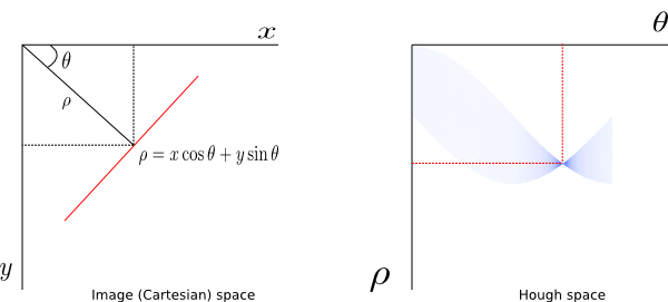
Fig. 1: Representation of a line in Cartesian (left) and Hough (right) coordinates.

The equation of the line can be modified to get its alternate representation as

,

where is the distance of the line from the origin and and is the angle of the vector, of least magnitude,  to the line. The transformed coordinate space which has and as its axes, as shown in right panel of the above figure, is called Hough space. A point in image space is mapped to a sinusoidal curve in Hough space. A set of points belonging to a line in image space get mapped to a set of sinusoids intersecting at a point in Hough space. So the problem of detecting a line in an image becomes a problem of detecting a point in Hough space. Once we detect the points in Hough space, we can do inverse transform to get the corresponding line in image space.

That’s it! We are ready for a simple demo.

A Simple Demo in Python

This demo is implemented in Python for algorithm explanation without paying attention to computational speed/optimization. We will apply Hough transform on Gantry crane image and extract first few strongest lines in the image. First of all, lets load the required libraries:

import numpy as N
import scipy.ndimage as I
import matplotlib.image as IM
import matplotlib.pyplot as plt

Next, we read the image using imread. The input RGB image is not a matrix (2D array). We would like to convert it into an image that can be represented as 2D array. We do so by converting the RGB image into grayscale image:

def rgb2gray(img_array):
  assert(img_array.shape[2] == 3)
  img_gray_array = N.zeros((img_array.shape[0], img_array.shape[1]), dtype=N.float32)
  for i in range(img_array.shape[0]):
    for j in range(img_array.shape[1]):
      img_gray_array[i][j] = 0.2989*img_array[i][j][0] + \
          0.5870*img_array[i][j][1] + 0.1140*img_array[i][j][2]
  return img_gray_array

The RGB image read using imread and corresponding grayscale image generated using the above given function rgb2gray are shown in Fig. 2 and Fig. 3, respectively.

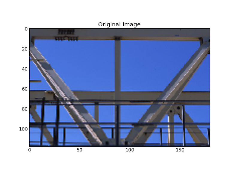
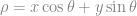
Fig. 2: Input image.

Fig.3: Grayscale image obtained from RGB image in Fig. 2.

Next, we would like to do some pre-processing on the grayscale image and get an image with few line or line-like features in it. There are several image preprocessing techniques that are applied to an image so that feature extraction becomes much easier. I am not going to clutter this simple post with explainations on noise reduction, thresholding, edge detection, etc. As an one-step solution, I am just binarizing the grayscale image with a hard threshold, that is, discard all the pixels with intensities lower than a specified value. Note that, we will lose several line-like features after this oversimplified binarization. This gives us the binarized image as shown in Fig. 4.

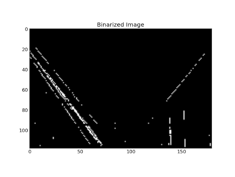
Fig. 4: Image obtained by binarizing image in Fig. 3

We can see that we have some line-like features in the binarized  image so that we can apply standard Hough transform to extract them. The advantage of using this binarized image is that we operate only on the white pixels (1’s) of the image. Now you can guess why people would like to apply pre-processing techniques before applying Hough transform on an image.

Computation of Hough transform is a simple voting procedure. We first define a  grid in Hough space. This grid is used to define an array called accumulator. The accumulator is simply a 2-D array that has same size as  grid. All the values in the accumulator are initialized to zero. Then, for each point in image space, we generate corresponding sinusoid in Hough space. For each   pair we get for a point in Hough space (the sinusoids are in Hough sapce), we quantize (bin) the values to the nearest points in the accumulator grid and increment the corresponding accumulator value by one. The process is repeated for all the points in image space. Following snippet of code might be more understandable than the mess of words:

def hough_transform(img_bin, theta_res=1, rho_res=1):
  nR,nC = img_bin.shape
  theta = N.linspace(-90.0, 0.0, N.ceil(90.0/theta_res) + 1.0)
  theta = N.concatenate((theta, -theta[len(theta)-2::-1]))

  D = N.sqrt((nR - 1)**2 + (nC - 1)**2)
  q = N.ceil(D/rho_res)
  nrho = 2*q + 1
  rho = N.linspace(-q*rho_res, q*rho_res, nrho)
  H = N.zeros((len(rho), len(theta)))
  for rowIdx in range(nR):
    for colIdx in range(nC):
      if img_bin[rowIdx, colIdx]:
        for thIdx in range(len(theta)):
          rhoVal = colIdx*N.cos(theta[thIdx]*N.pi/180.0) + \
              rowIdx*N.sin(theta[thIdx]*N.pi/180)
          rhoIdx = N.nonzero(N.abs(rho-rhoVal) == N.min(N.abs(rho-rhoVal)))[0]
          H[rhoIdx[0], thIdx] += 1
  return rho, theta, H

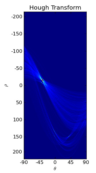
Fig.5: Hough transform of image in Fig. 4.

Figure 5 shows the final accumulator array (or Hough transform) obtained for our binary image. We can see several sinusoids interesecting at several places. Each such intersection corresponds to a line in image space. The image is in jet colormap, so more red the intersection point is, better is the line in image sapce. We can easily extract the intersection points and find corresponding values of pairs in Hough space from which we can compute the slope and y-intercept of the line in image space. That’s how we detect lines in an image using standard Hough transform.

I detected the two strongest intersection points in the Hough transform image and used the detected  values to generate lines in image space. Fig. 6 shows the detected lines overlaid in the binarized image.

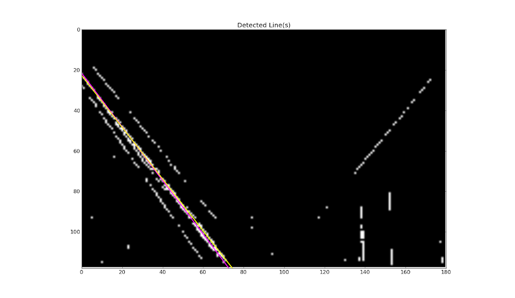
Fig. 6: Two detected lines (colored).

Conclusion

We learned to use standard Hough transform to detect lines in an image.